Page 37 - JSOM Winter 2024

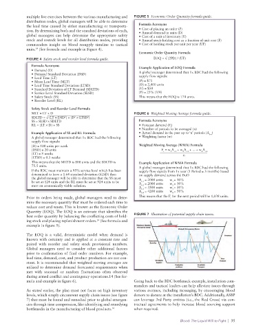
multiple live exercises between the various manufacturing and FIGURE 5 Economic Order Quantity formula guide.
distribution nodes, global managers will be able to determine
the lead time caused by either manufacturing or transporta- Formula Acronyms
tion. By determining both and the standard deviations of each, • Cost of placing an order (P)
global managers can help determine the appropriate safety • Annual demand in units (D)
• Cost of a unit of inventory (U)
stock and restock levels for all distribution nodes, providing • Annual stock-holding cost as a fraction of unit cost (F)
commanders insight on blood resupply timeline to tactical • Cost of holding stock per unit per year (UF)
units. (See formula and example in Figure 4).
14
Economic Order Quantity Formula
FIGURE 4 Safety stock and reorder level formula guide. EOQ = √ (2PD) / (UF)
Formula Acronyms Example Application of EOQ Formula
• Demand (D)
• Demand Standard Deviation (DSD) A global manager determined that 1x BDC had the following
• Lead Time (LT) supply flow signals:
• Mean Lead Time (MLT) (P) = $75
• Lead Time Standard Deviation (LTSD) (D) = 2,400 units
• Standard Deviation of LT Demand (SDLTD) (U) = $50
• Service Level Standard Deviation (SLSD) (F) = 25% (1/4)
• Safety Stock (SS) This means that the EOQ is 174 units.
• Reorder Level (RL)

Safety Stock and Reorder Level Formula
MLT = LT x D FIGURE 6 Weighted Moving Average formula guide.
2
2
SDLTD = √ (LT × DSD ) + (D × LTSD )
2
SS = SLSD × SDLTD Formula Acronyms
RL = (LT × D) + SS • Forecast demand (F ) t
• Number of periods to be averaged (n)
Example Application of SS and RL Formula • Actual demand in the past up to ‘n’ periods (A )
t-n
A global manager determined that 1x BDC had the following • Weighting factor (w)
supply flow signals:
(D) = 100 units per week Weighted Moving Average (WMA) Formula
(DSD) = 20 units F = w A + w A + ... + w A t-n
t-2
t
1
n
t-1
2
(LT) = 8 weeks n
(LTSD) = 0.5 weeks
This means that the MLTD is 800 units and the SDLTD is Example Application of WMA Formula
75.5 units. A global manager determined that 1x BDC had the following
If the BDC must maintain a 95% service level which has been supply flow signals from 1x year (1 Period = 3 months) based
determined to have a 1.64 standard deviation (SLSD) then on supply demand across the DoD
the global manager will be able to determine that the SS must A = 2000 units w = 10%
t-1
be set at 124 units and the RL must be set at 924 units to be A = 2000 units w = 10%
1
meet an economically viable solution. t-2 2
A = 3500 units w = 30%
3
t-3
A = 4200 units w = 50%
t-4 4
Prior to orders being made, global managers need to deter- This means that the F for the next period will be 1,038 units.
t
mine the necessary quantity that must be ordered each time to
reduce cost and waste. This is known as the Economic Order
Quantity (EOQ). The EOQ is an estimate that identifies the
best order quantity by balancing the conflicting costs of hold- FIGURE 7 Illustration of potential supply chain issues.
ing stock and placing replenishment orders. (See formula and
14
example in figure 5).
The EOQ is a valid, deterministic model when demand is
known with certainty and is applied at a constant rate and
paired with reorder and safety stock provisional numbers.
Global managers need to consider other additional factors
prior to confirmation of final order numbers. For example,
lead time, demand, cost, and product production are not con-
stant. It is recommended that weighted moving averages are
utilized to determine demand forecasted requirements when
met with seasonal or random fluctuations often observed
during armed conflict and contingency operations.14 (See for-
mula and example in figure 6). Going back to the BDC bottleneck example, installation com-
manders and tactical leaders can help alleviate issues through
As stated earlier, the plan must not focus on high inventory various avenues, including messaging, by encouraging blood
levels, which simply circumvent supply chain issues (see figure donors to donate at the installation’s BDC. Additionally, ASBP
7) that must be found and remedied prior to global emergen- can leverage 3rd Party entities (i.e., the Red Cross) via con-
cies through time compression, like identifying and remedying tractual agreements to help increase blood sourcing support
bottlenecks in the manufacturing of blood products. 14 when required.
Blood: The Liquid Will to Fight | 35