Page 44 - Journal of Special Operations Medicine - Spring 2014

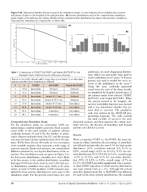
Figure 5 (A) Survival probability functions used in the simulation; height of curve indicates the probability that a patient
will survive if taken to the hospital at the indicated time. (B) Severity distributions used in the comprehensive simulation
study; height of bar indicates the relative likelihood that a patient in that distribution has injury characteristics classified as
Expectant (E), Immediate (I), Delayed (D), or Minor (M).
1
Delayed (A)
Immediate
0.9
(B)
0.8
Low Acuity Distributio n Random Distribution High Acuity Distribution
0.7 0.5 0.5 0.5
0.4 0.4 0.4
Probability of Survival 0.5 Probability 0.3 0.3 0.3
0.6
0.2
0.2
0.2
0.4
0.1 0.1 0.1
0.3
0 0 0
E I D M E I D M E I D M
Severity Severity Severity
0.2
0.1
0
0 20 40 60 T 80 100 120 140 160 180
Time since incident (minutes)
Table 1 Comparison of START, ReSTART, and Simple-ReSTART for the ambulance, we used a lognormal distribu-
Example Under Different Levels of Resource Scarcity. tion, which has previously been used to
model ambulance travel times. A Poisson
9
Entries in the table indicate which triage class is prioritized or at what time
priority switches from immediate to delayed. process was used to model the initial ar-
10
V S START ReSTART Simple-ReSTART rivals of the ambulances to the scene.
Using the same randomly generated
3 –83.0 Immediate Delayed Delayed travel times for each of the three models,
6 –8.0 Immediate Delayed Delayed we simulated the hospital arrival times of
9 17.0 Immediate Switch @ 17 min Delayed the patients under three policies: START,
12 29.5 Immediate Switch @ 29.5 min Delayed ReSTART, and Simple-ReSTART. When
the patient arrived at the hospital, the
15 37.0 Immediate Switch @ 37 min Immediate survival probability function was checked
18 42.0 Immediate Switch @ 42 min Immediate and it was determined whether that pa-
21 45.6 Immediate Immediate Immediate tient died or survived. The simulation
code was written in the MATLAB pro-
24 48.3 Immediate Immediate Immediate
gramming language. The code counted
the total number of survivors for each
Comprehensive Simulation Study simulated scenario and then reported the critical mor-
For the simulation study, we constructed 3,000 sce- tality rate (i.e., the fraction of immediate and delayed
narios using a random number generator. Each scenario patients who did not survive).
could differ in the total number of patients (chosen
randomly between 25 and 125), the number of ambu-
lances (chosen randomly from 2 to 15), and the average Results
one-way trip time (chosen randomly from 10 to 45 min- When comparing START vs. Re-START, the mean de-
utes). While these choices obviously do not encompass crease in critical mortality, the percentage of immediate
every possible scenario, they represent a wide range of and delayed patients who die, was 8.5% for high- acuity
resource scarcity. From each scenario, we created three distribution (95% confidence interval [CI] 8.3% to
different incidents by varying the distribution of the ca- 8.8%, overall range –2.2% to 21.1%), 9.3% for uni-
sualties. The distributions used are given in Figure 5: in form distribution (95% CI 9.0% to 9.6%, overall range
the low-acuity distribution, casualties were more likely –0.2% to 21.2%), and 9.1% for low-acuity distribu-
to be less severe; in the random distribution, casualties tion (95% CI 8.9% to 9.4%, overall range –0.7% to
had equal likelihood of any severity; and in the high-acu- 21.1%). ReSTART provided significantly lower mortal-
ity distribution, casualties were more likely to be more ity than START regardless of which severity distribution
severe. A total of 9,000 incidents (3,000 scenarios mul- was used (paired t test, p < .01). Although the critical
tiplied by three severity distributions) were used in the mortality improvement due to ReSTART was different
simulation study. For the per-trip travel times for each for each of the three severity distributions, the nominal

36 Journal of Special Operations Medicine Volume 14, Edition 1/Spring 2014